Statistics - Normal Distribution
The normal distribution is an important probability distribution used in statistics.
Many real world examples of data are normally distributed.
Normal Distribution
The normal distribution is described by the mean (\(\mu\)) and the standard deviation (\(\sigma\)).
The normal distribution is often referred to as a 'bell curve' because of it's shape:
- Most of the values are around the center (\(\mu\))
- The median and mean are equal
- It has only one mode
- It is symmetric, meaning it decreases the same amount on the left and the right of the center
The area under the curve of the normal distribution represents probabilities for the data.
The area under the whole curve is equal to 1, or 100%
Here is a graph of a normal distribution with probabilities between standard deviations (\(\sigma\)):
- Roughly 68.3% of the data is within 1 standard deviation of the average (from μ-1σ to μ+1σ)
- Roughly 95.5% of the data is within 2 standard deviations of the average (from μ-2σ to μ+2σ)
- Roughly 99.7% of the data is within 3 standard deviations of the average (from μ-3σ to μ+3σ)
Note: Probabilities of the normal distribution can only be calculated for intervals (between two values).
Different Mean and Standard Deviations
The mean describes where the center of the normal distribution is.
Here is a graph showing three different normal distributions with the same standard deviation but different means.
The standard deviation describes how spread out the normal distribution is.
Here is a graph showing three different normal distributions with the same mean but different standard deviations.
The purple curve has the biggest standard deviation and the black curve has the smallest standard deviation.
The area under each of the curves is still 1, or 100%.
A Real Data Example of Normally Distributed Data
Real world data is often normally distributed.
Here is a histogram of the age of Nobel Prize winners when they won the prize:
The normal distribution drawn on top of the histogram is based on the population mean (\(\mu\)) and standard deviation (\(\sigma\)) of the real data.
We can see that the histogram close to a normal distribution.
Examples of real world variables that can be normally distributed:
- Test scores
- Height
- Birth weight
Probability Distributions
Probability distributions are functions that calculates the probabilities of the outcomes of random variables.
Typical examples of random variables are coin tosses and dice rolls.
Here is an graph showing the results of a growing number of coin tosses and the expected values of the results (heads or tails).
The expected values of the coin toss is the probability distribution of the coin toss.
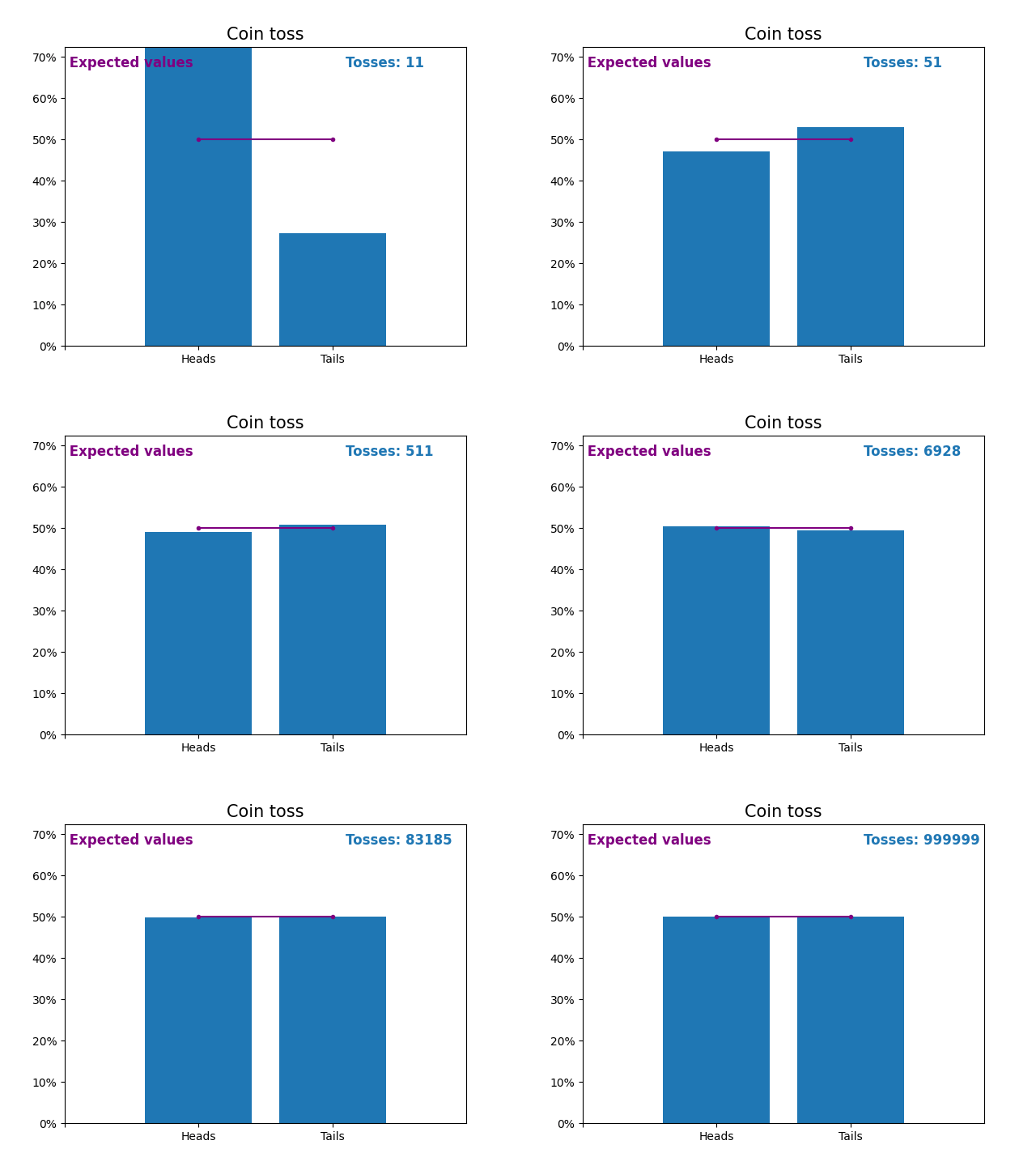
Notice how the result of random coin tosses gets closer to the expected values (50%) as the number of tosses increases.
Similarly, here is a graph showing the results of a growing number of dice rolls and the expected values of the results (from 1 to 6).
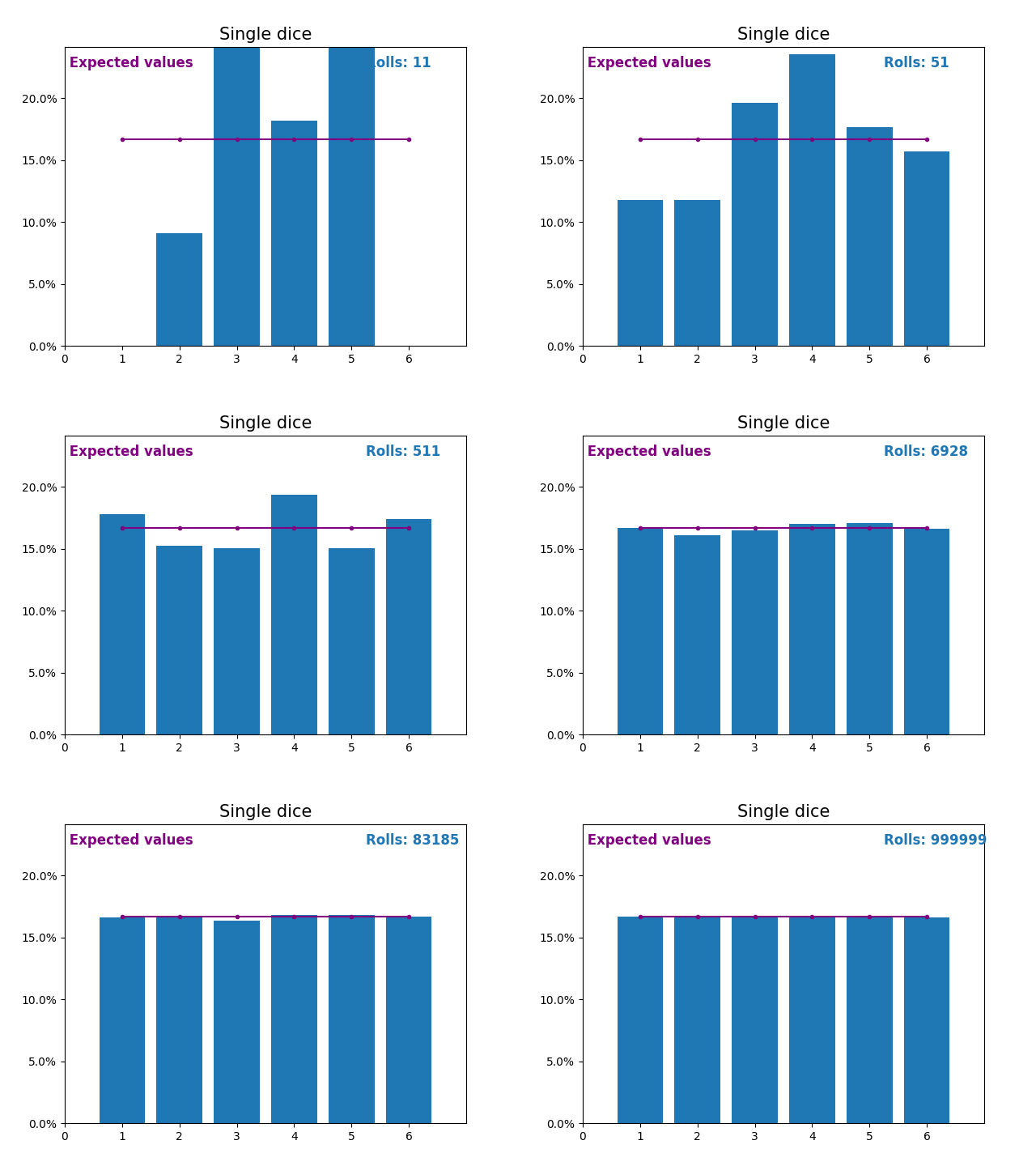
Notice again how the result of random dice rolls gets closer to the expected values (1/6, or 16.666%) as the number of rolls increases.
When the random variable is a sum of dice rolls the results and expected values take a different shape.
The different shape comes from there being more ways of getting a sum of near the middle, than a small or large sum.
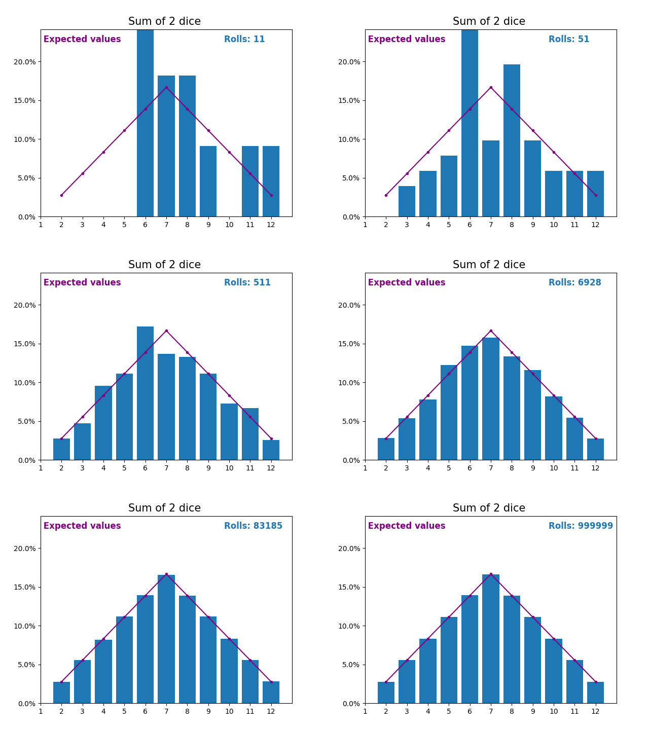
As we keep increasing the number of dice for a sum the shape of the results and expected values look more and more like a normal distribution.
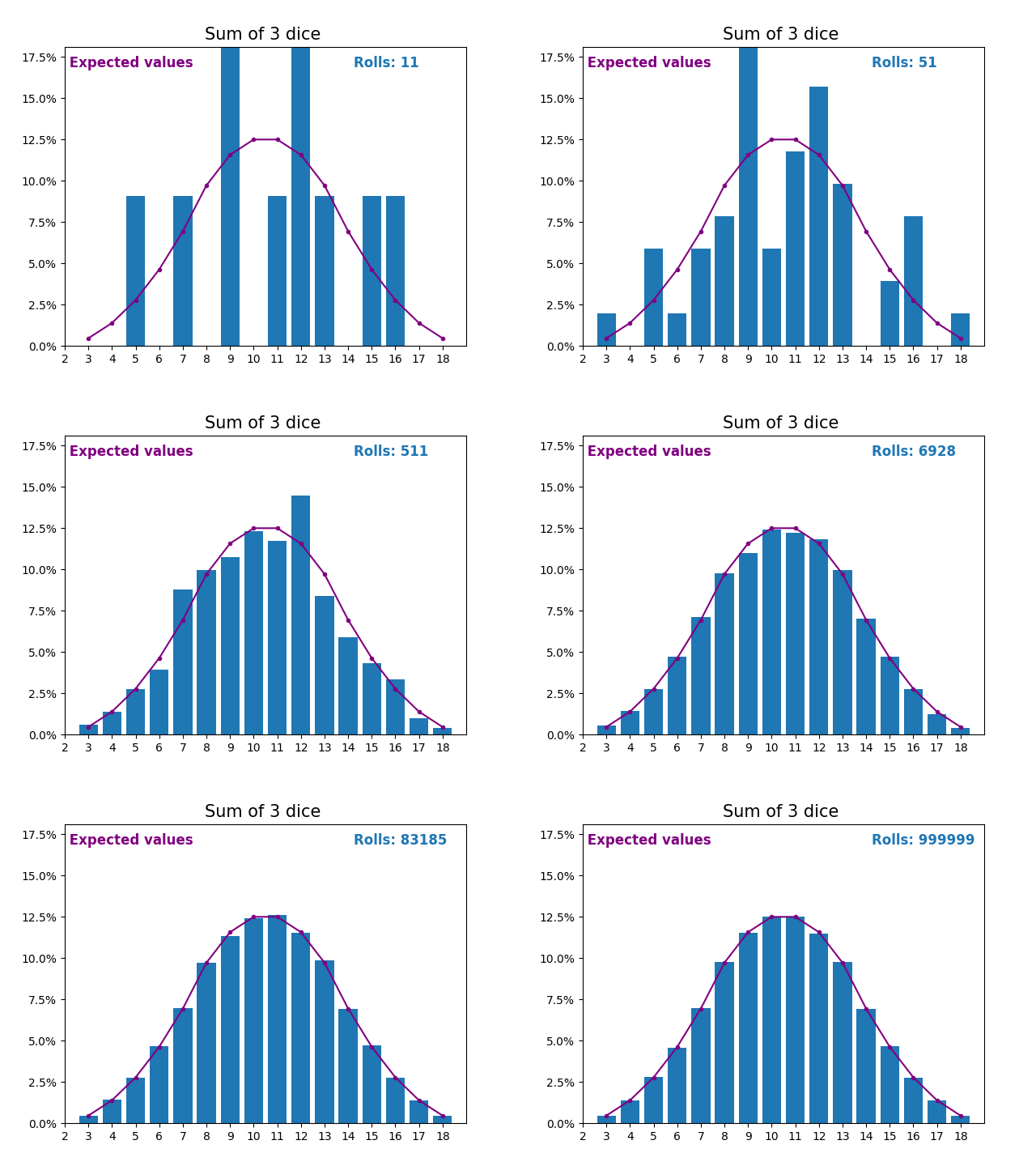
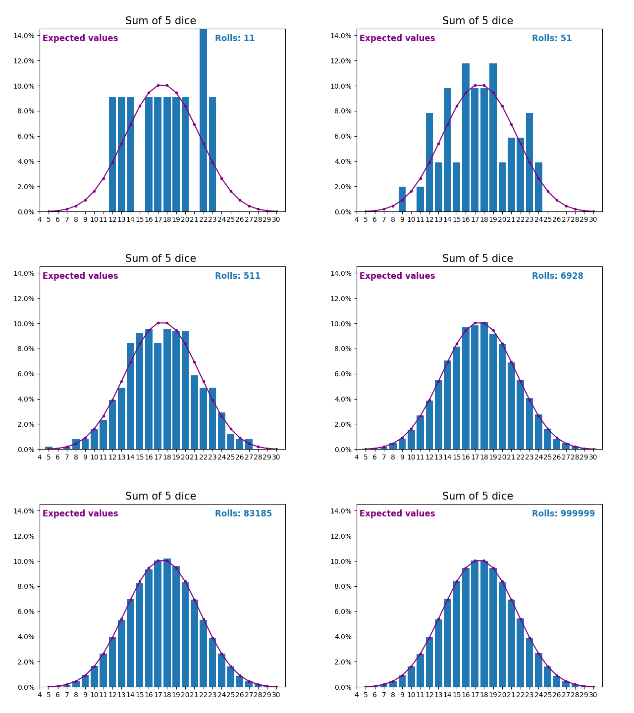
Many real world variables follow a similar pattern and naturally form normal distributions.
Normally distributed variables can be analyzed with well-known techniques.
You will learn about some of the most common and useful techniques in the following pages.


