Google Sheets Conditional Formatting
Conditional Formatting
Conditional formatting is used to change the appearance of cells in a range based on your specified conditions.
The conditions are rules based on specified numerical values, matching text and more.
Changing the appearance of cells can visually highlight interesting data points for analysis.
Google Sheet provides a number of preset formatting options, as well as customizable format options and conditions.
The two main Conditional Formatting options are:
Single Color formatting applies a single customizable formatting option to all the cells that match a condition.
Color Scale formatting applies a background color that smoothly changes between 2 or 3 colors based on the values of cells in a range.
Note: Single Color formatting lets you customize both the background color and the font in the cells.
Conditional Formatting Example
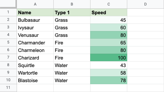
Here, the Speed values of each pokemon is formatted with a Color Scale:

Note: Google Sheets can customize the color and behaviour of color scale conditional formatting.
Clear Formatting
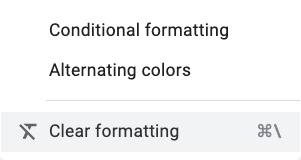
Conditional Formatting can be removed by selecting the range of cells you want to remove the conditional formatting from and selecting the Clear formatting option from the Format menu:

Note: You can read more about removing formatting in the Clear Format chapter.
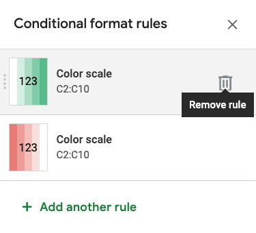
Rules can also be removed in the right-hand side Conditional format rules menu.
Manage Formatting
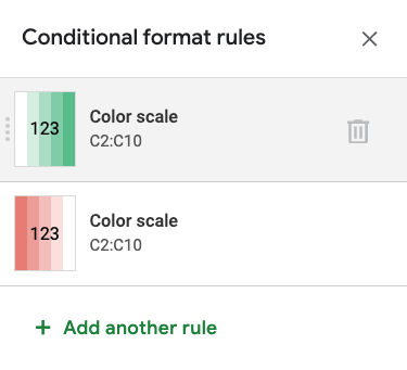
Conditional Formatting can be managed in the right-hand menu.
The menu is accessed by selecting the range of cells that already have conditional format rules and selecting Conditional format from the Format menu.

From this menu you can add extra rules:

You can remove rules by clicking the recycling bin icon:

Click the four vertical dots on the left of a rule and drag up or down to rearrange the rules:

Note: The rule at the top of the list is the one that will be applied.


