Excel HCR - Less Than

Highlight Cell Rules - Less Than

Highlight Cell Rules is a premade type of conditional formatting in Excel used to change the appearance of cells in a range based on your specified conditions.

Less Than... is one of the options for the condition.

Here is the Highlight Cell Rules part of the conditional formatting menu:

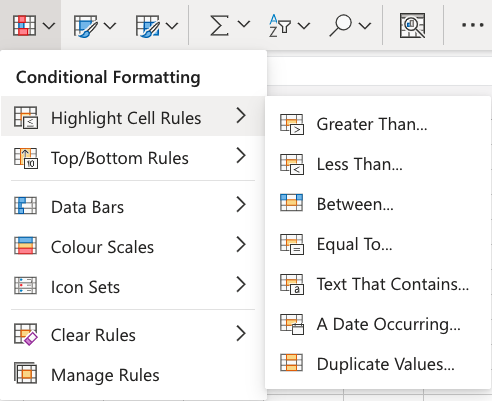
Highlight Cell Rule - Less Than Example

The "Less Than..." Highlight Cell Rule will highlight a cell with one of the appearance options based on the cell value being less than to your specified value.

The specified value is typically a number, but it also works with a text value.

In this example, the specified value will be "55".

Name Type 1 HP Attack Defense Sp. Atk Sp. Def Speed Magikarp Water 20 10 55 15 20 80 Gyarados Water 95 125 79 60 100 81 Lapras Water 130 85 80 85 95 60 Ditto Normal 48 48 48 48 48 48 Eevee Normal 55 55 50 45 65 55 Vaporeon Water 130 65 60 110 95 65 Jolteon Electric 65 65 60 110 95 130

Copy Values

You can choose any range for where the Highlight Cell Rule should apply. It can be a a few cells, a single column, a single row, or a combination of multiple cells, rows and colums.

Let's apply the rule to the Attack values.

"Less Than..." Hightlight Cell Rule, step by step:

1. Select the range D2:D8 for Attack values

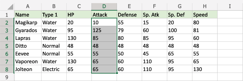
2. Click on the Conditional Formatting icon in the ribbon, from Home menu
3. Select the Highlight Cell Rules from the drop-down menu
4. Select the Less Than... from the menu

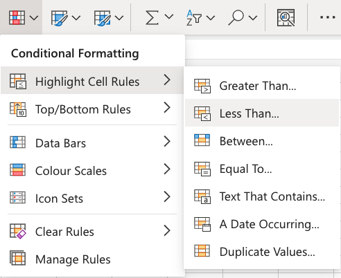
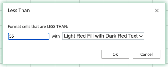
This will open a dialog box where you can specify the value and the appearance option.

5. Enter 55 into the input field
6. Select the appearance option "Light Red Fill with Dark Red Text" from the dropdown menu

Now, the cells with values less than "55" will be highlighted in red:

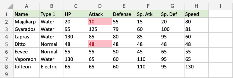
Only Magikarp and Ditto have Attack values less than 55, so these values are highlighted.

Highlight Cell Rule - Less Than Example (with Text)

The "Less Than..." Highlight Cell Rule also works with text values.

Excel will use alphabetical order (A-Z) to highlight the text values that starts with a letter that is earlier in the alphabet than the specified value

In this example, the specified text value will be "Electric".

Name Type 1 HP Attack Defense Sp. Atk Sp. Def Speed Magikarp Water 20 10 55 15 20 80 Gyarados Water 95 125 79 60 100 81 Lapras Water 130 85 80 85 95 60 Ditto Normal 48 48 48 48 48 48 Eevee Normal 55 55 50 45 65 55 Vaporeon Water 130 65 60 110 95 65 Jolteon Electric 65 65 60 110 95 130

Copy Values

You can choose any range for where the Highlight Cell Rule should apply. It can be a a few cells, a single column, a single row, or a combination of multiple cells, rows and colums.

Let's apply the rule to the Type 1 values.

"Less Than..." Hightlight Cell Rule, step by step:

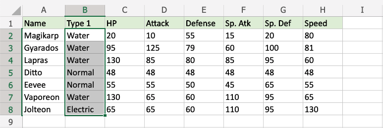
1. Select the range B2:B8 for Type 1 values

2. Click on the Conditional Formatting icon in the ribbon, from Home menu
3. Select the Highlight Cell Rules from the drop-down menu
4. Select the Less Than... from the menu

This will open a dialog box where you can specify the value and the appearance option.

5. Enter Electric into the input field
6. Select the appearance option "Yellow Fill with Dark Yellow Text" from the dropdown menu

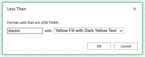
Now, the cells with text values earlier in the alphabet than "Electric" will be highlighted in yellow:

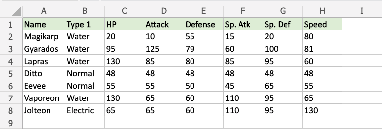
Nothing seems to have changed!

Water starts with "W" and Normal starts with "N".

"W"and "N" are all later in the alphabet than "E", which Electric starts with, so none of these are highlighted.

So, what about the rest of the letters in the text value?

Let's see what happens if we add a fictional pokemon with a new Name and Type:

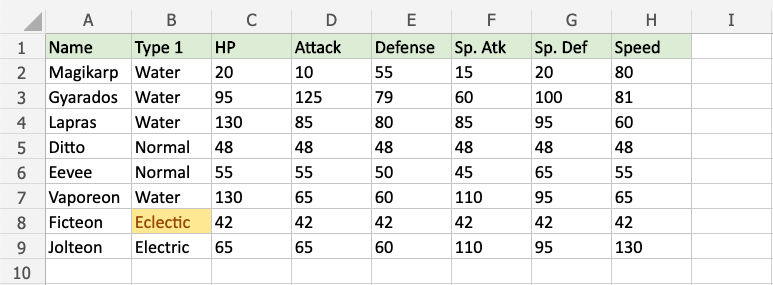
Notice that the fictional "Ficteon" has the type "Eclectic", which is highlighted.

The Excel condition checks each letter in the specified text value from left to right.

Because the "c" in "Eclectic" comes earlier in the alphabet than the "l" in "Electric", this is considered Less Than and is highlighted.